OpenAI o1 Technology Series 1: Overall Framework, Utilizing Test Time Scaling Law to Enhance Logical Reasoning Ability

The o1 model launched by OpenAI a few days ago, with its significantly improved logical reasoning ability, has sparked heated discussions about the training methods behind it. The introduction and output result demo of o1 will not be elaborated here. You can go to the official website of OpenAI to read it (it is very short and easy to read because the secrets are all hidden). I believe that in recent times, when people explore online how o1 is trained, they will definitely come across the following hot topics:

• Test/Inference-Time scaling law， Enhance the inference capability of the model by increasing the computational power in the inference stage

• Post Training， Improve the reasoning ability of the model through post training

• PRM/ORM: Process/Outcome Based Reward Model

• CoT: Chain of Thinking

• Reinforcement learning, self play, and MCTS (Monte Carlo Search Tree Algorithm) ）

wait.

When these words appear individually in front of us, it seems difficult for us to string them together. Not only that, but we also don’t know the principles behind individual words, such as “what is test/reference time scaling law”? What does it mean to spend computing power on the inference stage? Why does spending computing power on the inference stage lead to better results? What is its relationship with post training? Such things make it difficult to imagine a complete flowchart in one’s mind.

During my exploration of O1, I referred to this GitHub repository（ https://github.com/hijkzzz/Awesome-LLM-Strawberry ） Inside, various materials related to the algorithms behind O1, including relevant papers, code, and Twitter posts, have been collected from both internal and external sources. Among them, there are many research achievements of o1 core contributors in recent years. After reading these materials, I found that they can be divided into 2 points:

• Framework research results It can be understood as the generalized framework behind the o1 training algorithm. It introduces some basic ideas such as Test/Reference Time Scaling law and provides some simple and universal practical solutions.

• Research results on the variation of details into categories It can be understood as an algorithm variation that is nested within the framework or inspired by the framework in terms of practical details (but not necessarily published later than the framework). In summary, each family has its own approach.

And this article focuses on a detailed interpretation and development of framework research results, I have selected 2 articles that I believe can be considered as frameworks They are:

• Let’s Verify Step by Step  （OpenAI）

• Hunter Lightman, Vineet Kosaraju, Yura Burda, Harri Edwards, Bowen Baker, Teddy Lee, Jan Leike, John Schulman, Ilya Sutskever, Karl Cobbe

• Scaling LLM Test-Time Compute Optimally can be More Effective than Scaling Model Parameters (Google Deepmind)

• Charlie Snell, Jaehoon Lee, Kelvin Xu, Aviral Kumar

This article will be based on the second article, while interspersing the core content of the first article for explanation. There will be a separate interpretation of ‘lets verify step by step’ in the future. In the later articles, I will select the research results of various types of details that I find interesting, such as algorithms that may have some similarities with O1, and conduct in-depth analysis with the source code (as long as they have it).

Finally, both of these articles are of a type that is generally easy to read, but difficult to grasp in terms of details. Therefore, I have tried my best to interpret the details based on my own experience, striving to restore all aspects of the training. At the same time, I have disassembled the original paper and tried to better explain it from a framework perspective . Before reading this article, it is recommended that you first review the demo of the output results in the openai o1 technical report to better understand what the “model thinking process” is

1、 What is Test/Reference time Scaling Law

Imagine if we have a basic model (we call it a generator) in our hands, but its logical reasoning ability (such as the ability to solve mathematical problems) is poor, how can we improve it? To be more specific, without considering the cost associated with the dataset, assuming my GPU computing power (FLOPs) is limited, how can I utilize it to enable my model to ultimately infer better results?

A more direct idea is to invest computing power in its maintenance phase and inject more pre training knowledge of mathematical logic into the model . For example, using better and more mathematical data, or expanding the parameter scale of the model. This approach is inspired by the well-known scaling law (more specifically, the pretrain time scaling law).

However, When we study the technical report of OpenAI O1, we will find that it has used this computing power more in two areas:

• Used in RLHF training (post training)

• Used in the inference phase of the model (Test/Affeece)

For details, please refer to the image drawn in the o1 report:

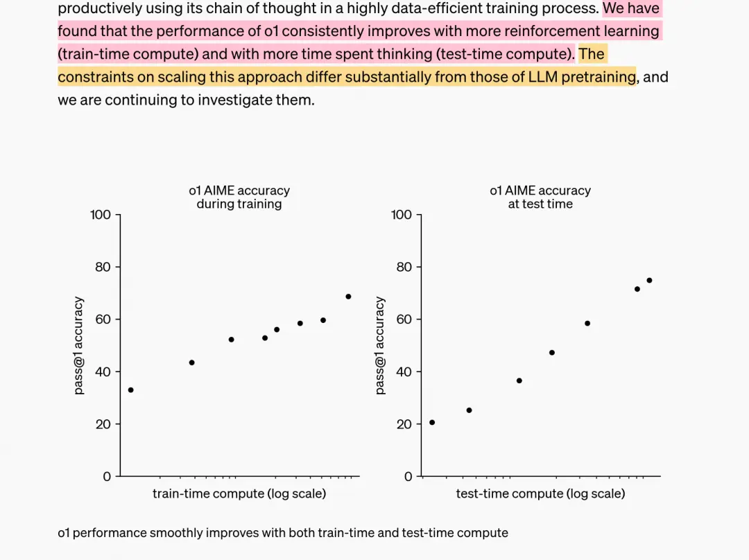
• Once, in order to improve the logical reasoning ability of the model, we spent all our computing power on the pretrain stage, thus giving birth to the pretrain scaling law

• Now, there are ready-made product proofs that if computing power is spent on post training and inference, the inference ability of the model will be greatly improved, indicating the existence of a Test/Affeece scaling law.

• Just as the pre training scaling law is influenced by model parameters and training data, the Test/Affeece scaling law is also inevitably affected by certain factors, and what these factors are and how they affect them are the topics that this article aims to explore.

But wait, at this moment you must want to ask:

• Question 1: Generally speaking, the effectiveness of a model is determined by its training stage, so if we talk about improving the model’s reasoning ability through pretraining or post training, I can understand. But how does the inference stage improve the reasoning ability of the model? What do you mean by using computing power in the inference stage?

• Question 2: Are post training and inference two independent methods for improving model inference ability? Can they be used together?

Let’s answer these two questions step by step.

Use computing power in the inference stage, which means improving the final generation performance of the model by optimizing the inference method without moving the model we have already trained. There are two situations here.

• Optimize reasoning input

• Optimize reasoning output

1.1 Optimize inference input: prompt

This method should be very familiar to everyone. For example, it turns out that your model eats a question and directly spits it out for you to answer. But now in order for the model to better simulate human thinking, if you want the model to think step by step before giving an answer, that is, the generated results of the model include the thinking steps and answers, then you can choose to give the model corresponding examples in the prompt, or guide the model to think step by step in multiple rounds of dialogue to achieve this goal. Related papers can be found at:

• Chain-of-Thought Prompting Elicits Reasoning in Large Language Models

• Jason Wei, Xuezhi Wang, Dale Schuurmans, Maarten Bosma, Brian Ichter, Fei Xia, Ed Chi, Quoc Le, Denny Zhou

The more details your prompt provides and the more rounds of guidance you provide, the better the model may produce. And more tokens mean that the inference stage requires more computing power, so this is one of the specific contents of what we call ‘spending computing power on the inference stage can improve model performance’.

1.2 Optimize inference output: revise output distribution

However, the method of optimizing inference input is still not direct enough. Do I need to carefully design prompts or manually induce the model to think step by step for every problem. So can we make the model automatically perform the CoT process after solving a problem?

That is to say, we now hope that the model can autonomously generate the following outputs after eating the next question:

attempt1 -> attempt2 -> attempt3 -> ...-> attempti -> answer

Among them, each attempt contains “multiple intermediate steps+final answer”, which simulates the human thinking process: first make one attempt, then discover the problem, and on this basis, make other attempts until the final answer is found.

So how can I make the model achieve this? An intuitive way is, if I have:

problem -> attempt1 -> ... -> attempti -> answer

Can’t I train directly with this labeled data? There are also many training methods, such as:

• Solution 1: I directly do SFT, place the most correct attempt at the end of the input sequence, and use it as a label for training

• Solution 2: I use a method similar to RLHF. First, I have a reward model that can evaluate each thinking step. Then, using this evaluation result, I guide the model to search step by step, finding the best thinking step for each step. Finally, I can find the answer?

These two solutions, From the perspective of training methods alone, it can be considered as post training That is to say, we improve the logical reasoning ability of the model by investing computing power in post training.

But isn’t the title of this article ‘Spending Computing Power on Inference’? Where is the inference? Let’s re-examine these two solutions again ：

• Assuming we have trained the model using either Solution 1 or Solution 2 post training, we will now use it for inference. The model takes a question and produces a series of intermediate results and answers, But can you guarantee that these intermediate results and answers are always the best?

• At this point, if we could have a verifier to evaluate the quality of intermediate steps (such as the reward model in Solution 2), would we be able to better guide the model to produce better results step by step when using these post trained models for inference ？ For example, we sample multiple attempts chains for a problem and find the best one from them. Or find the best attempt within a single attempt, and so on.

• Or, suppose we are in the post training stage, using this verifier to guide the model automation Generate high-quality training data (this is an inference step), and based on this data, we perform alignment. So perhaps we can directly trust the results of post training.

So, for the part of optimizing inference output, you can spend all your computing power on post training or on post training+inference. From the technical report of o1, it should have chosen the latter, while post training has chosen some reinforcement learning based approach（ In fact, there should also be changes in O1 during the pretrain stage. We will provide a hypothesis based on experimental data in the following analysis ）. So far, we have answered both question 1 and question 2 clearly.

On the basis of understanding these, we roughly know [Framework] What does it look like, specifically:

1. Firstly, we need to guide the model from “only producing results” to “simultaneously producing intermediate steps and results”, a process called post training. During this process, you can use reinforcement learning based techniques or just fine tune SFT. You can either focus only on whether the model follows the format (i.e. only on whether intermediate results are produced without considering the quality of intermediate results), or you can focus on both the format and the quality of intermediate results at the same time

2. Secondly, we need to train a verifier that can evaluate intermediate results, which is actually a part of post training. This verifier can be used in post training based on reinforcement learning (although it may not be the only value assessment model), as well as guiding the search in the inference stage of step 3.

3. Next, we need to design a search method. It can evaluate scores based on the intermediate results returned by the verifier, and better guide the model to perform step-by-step searches during the inference stage, in order to achieve optimization in every step of thinking. If in the post training stage, you only focus on format, then applying this search method in the inference stage can better guide search results; if you have already focused on format+quality, this method can still achieve a higher level of effectiveness. Meanwhile, it should be noted that if we have already used a reinforcement learning based approach in the post training stage, this search method can also be applied to the stage of model production of “empirical data”, which can On the basis of self production and self consumption, dynamically screen high-quality datasets and then align them (Avoiding human annotations is not necessary, but if done well, inference may only need to be used in the post training stage to screen high-quality data, without the need to use it again after post training.).

With an understanding of the framework, let’s now take a look at the two solutions DeepMind has developed based on this framework:

• Method 1: Use PRM (Process enhanced Reward Model) to guide search

• Post training: Only guide the model to align formats+train a process based verifier (PRM)

• Inference: Use PRM to guide search

• Method 2: Directly changing the output distribution of the model through SFT (Revise proposal distribution)

• Post training: guiding alignment format through SFT, ensuring basic quality of intermediate results, and training process based verifier (PRM), which directly uses the PRM in scheme one.

• Inferce: Use PRM to guide search

Among them, Plan One focuses on exploring the general methods of training PRM and the design of the search process. Option two provides an example of SFT type post training. If we only look at the original paper, we can easily understand these two schemes as two aspects of the Test/Reference scaling law. But based on our summary of the framework, we can find that they actually talk about the same thing, only with different emphasis in their descriptions.

[Note] ⚠️⚠️： This section breaks the logical structure of the original paper and contains a lot of subjective understanding from the author. Please read it selectively

2、 Method 1: Use PRM to guide search

The main purpose of this method is to train a The Process Enhanced Reward Model (PRM) is capable of evaluating process data, which corresponds to the Results Based Evaluation (ORM), outcome-supervised Reward Model） To guide the model to better search for the best answer during the inference phase. The specific steps are as follows:

• Format training First, perform SFT on the model to produce results with process data

• Training PRM Train a verifier capable of evaluating the process, which we call PRM

• Using PRM to guide the search process Using the trained PRM, guide the model to search for the best answer.

Let’s take a closer look at these three points.

2.1 Format Training

For a basic model that does not perform any processing, when we feed it a question, it usually directly spits out the answer to us.

Now, we hope to guide the model to spend more time “thinking” before giving an answer, that is to say, we hope the model returns a response to us in the format of “thinking steps+answer”.

So here we need to format the model finely first. The specific method is:

• Self-produced data Add format examples in the prompt to guide the model to produce results in the format we want. For example, we can require the model to follow a line by line thinking step (as discussed in the paper ‘lets verify step by step’). We will add these results to the SFT dataset

• sftUsing this batch of automated SFT datasets, fine tune the model to generate data in a “thought process+answer” manner when answering questions in the future.

Note that this SFT process only focuses on format fine-tuning and does not pay attention to the quality of the thinking steps . The quality of the thinking steps is something we need to consider in the subsequent process.

2.2 Training PRM

Now, our model is able to generate ‘thinking steps’ data in the generated results. We need to train a reward model that can evaluate these steps, that isPRM（Process-supervised Reward Model）。

With ‘supervised’, it is necessary to have labeled data, which means that for each step, we need to give it a true value rating . So based on whether you are a super rich person, a wealthy person, or an average wealthy person (those who can be trained are not considered poor), we have different construction methods.

(1) Super Rich People

• Directly call the format adjusted model, feed it a wave of questions, and generate a wave of “steps+answers” data (with a huge amount of data)

• Ask manual labeling of steps (e.g. positive/negative/neutral).

This method seems to have no other drawbacks besides being expensive and time-consuming.

(2) Rich people

Compared to roughly packaging a bunch of data for manual annotation, can we use some form of detail filtering to only send the data we consider valuable for manual annotation?

• Directly call the format adjusted model, feed it a wave of questions, and generate a wave of “steps+answers” data (with a small data volume)

• Filter out some data containing ‘invalid answers’. For example, answers that cannot be parsed (such as LaTeX formulas that cannot be parsed, etc.). Note that ‘Invalid!=Error’

• Ask manual labeling of steps (e.g. positive/negative/neutral)

• Train a round of PRM using the currently annotated data

• Decide how to use PRM results to give an overall score for “steps+answers”, for example:

• Prod (continuous multiplication) PRM will score each step (under discrete labels, this score represents probability). We multiply the scores of all steps to represent the overall score

• Minimum formula (min) Take the minimum score among all steps as the overall score. This is because intuitively, if one step in steps goes wrong, the entire logical chain is likely to have problems. So we take the worst-case scenario as the overall score.

• The last step: When you train PRM, you definitely don’t feed a single step to PRM for scoring, but feed all steps together to give them contextual relationships (PRM needs to judge the score of the current step based on the previous steps) . So theoretically, taking the score of the last step can also reflect the overall score.

• Prod and Min are both methods explored by openAI in “lets verify step by step”, while Last step is the method used by DeepMind in this article. There is no absolute good or bad among these methods, it depends on how you design the entire training process (we will come back to this point later). We only emphasize the need to establish a rule that can map the single step scoring of PRM to the overall scoring

• Call the model again and generate a wave of data. Call the current version of PRM and use the overall scoring rule mentioned above to score the “steps” of a problem as a whole. We have specially selected the concatenating wrong answer data (with a high overall score, but the final answer is incorrect), and only sent these data to manual annotation . The reason for choosing this biased data is because they are confusing to the current PRM.

• Repeat the above process and iteratively train PRM

In summary, this method also requires manual annotation, but by filtering the dataset, the money is spent wisely.

(3) 【 Ordinary Rich People 】 (Key Focus)

In this case, we don’t need to manually label the data at all, which means The true value label of each step’s value is also estimated by us through some automated method So, how do we do it specifically?

• Directly call the format fine tuned model, feed it a wave of questions, and generate a wave of “steps+answers” data (depending on the data size needed)

• More specifically, for each problem, we sample N samples (In DeepMind settings, N=16, one sample is equivalent to one “steps+answer”)

• Filter out some data containing ‘invalid answers’. For example, answers that cannot be parsed (such as LaTeX formulas that cannot be parsed, etc.). Note that ‘Invalid!=Error’

• We estimate the value of each step using N Monte Carlo rollouts . The DeepMind article does not provide specific operational methods. Here, based on my experience, I can guess a possible implementation approach:

• sample”step1 -> step2 -> step3 -> answer”，step1~step3

• Taking step 1 as an example, we take it as the starting point (meaning problem+step 1), and then continue sampling N samples. It simulates N scenarios of ‘starting from step 1 and producing answers’.

• We calculate the proportion of solutions that can provide the correct answer. This ratio serves as the estimated value label for step 1.

• Since this label only indicates the possibility of finding the correct answer from the current step, it does not directly indicate that the current step is posterior/negative/neutral. Therefore, this label is also known as a “soft label”.

• For steps 2 and 3, we also estimate their value in the same way

• With this step soft label that we have automatically simulated, we can use it to train PRM models . In the settings of DeepMind, PRM is still a binary classification model, but the truth labels are not discrete when calculating loss.

2.3 Using PRM to guide the search process

So far, we have the following models:

• A model (generator) that can generate intermediate thinking steps according to a format However, the quality of the intermediate thinking steps cannot be guaranteed

• A reward model PRM (verifier) that can evaluate intermediate thinking steps . Once again, it should be emphasized that when we feed data to PRM for evaluation, we are not feeding only a single step, but the complete “problem+steps” data, because there is a contextual relationship between logical thinking steps.

And now what we want to do is:

• How to use a verfier to guide the generator to search for the best “steps+answer” without further training?

That is to say, we don’t want to spend extra computing power (FLOPs) on the training of the generator itself. We hope to invest computing power in the reasoning stage, using longer and more complex reasoning processes (manifested in the generator as longer “thinking” time), so that the generator can find the best answer.

So, next, we will provide a detailed introduction and analysis of three commonly used search schemes . The following figure provides an overview of these three options. Next, we will provide a detailed introduction to the implementation details of these three search schemes and analyze their effectiveness.

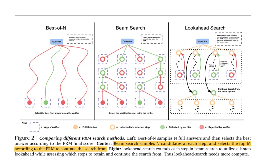
Here’s an additional note: once PRM is trained, we also need to develop a rule function that maps the single step scoring of PRM to the overall score That is to give an overall rating for a certain “steps+answer” under a question. On this basis, let’s do the search again. As mentioned in the previous text, you can go back and read the details（ Deepmind uses the last step scoring method, so in the following introduction, we will assume that the overall scoring method of PRM is this way ）。

（1）Best-of-N

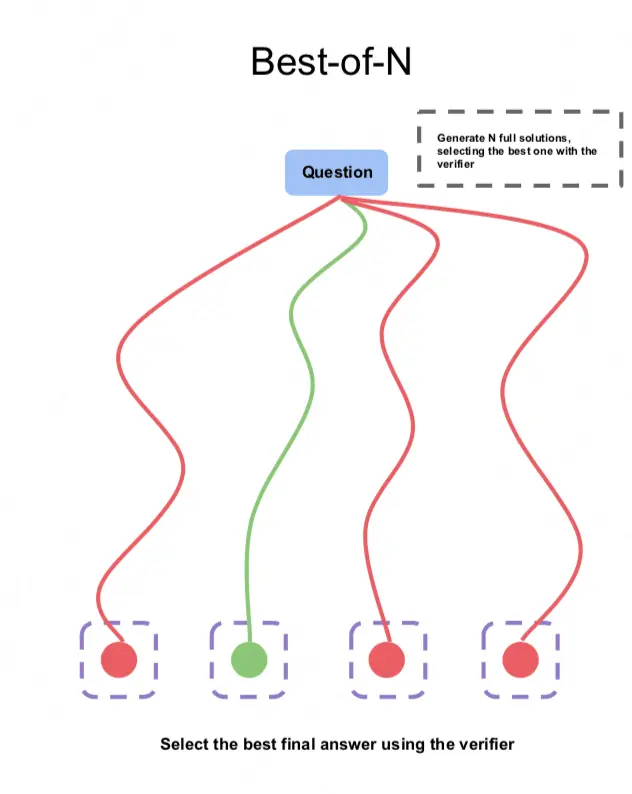
Due to its simplicity and intuitiveness, the accuracy of the answers obtained by the Best-of-N scheme is often used as a baseline for comparison with other schemes . The specific plan for Best-of-N is as follows:

• For a problem, we sample N samples (a single sample=steps+answer)

• Call PRM to score the intermediate steps of these N samples as a whole . The commonly used scoring methods include prod, min, and last step (as mentioned earlier)

• Select the group of steps+answer with the highest overall score as the output

There is also a slightly improved, weighted version of Best-of-N weighted method (The introduction provided by Deepmind is relatively vague, so the following introduction contains some of the author’s hypotheses):

• For a problem, we sample N samples (a single sample=steps+answer)

• Check the answers for these N samples. Assuming these samples provide a total of three types of answers, x, y, and z, with a, b, and c answers under each answer (N=a+b+c)

• So for the sample with the answer x, its final score=(a/N) * the overall score given by PRM. A/N is called weight.

(2）Beam Search

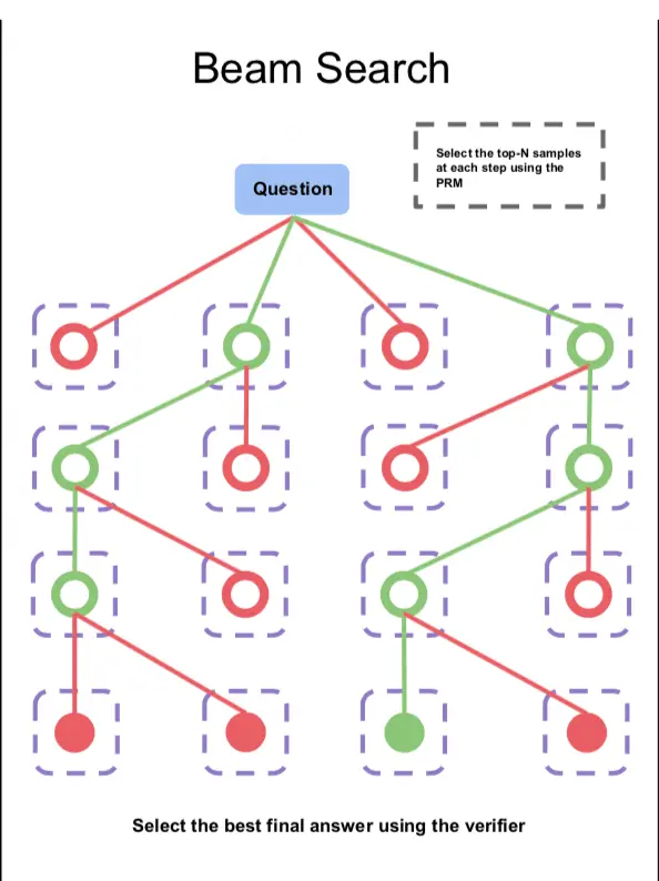
• For a problem, we first sample N steps 1 in parallel (e.g. N=4 in the above figure)

• Send each ‘question+step 1’ into PRM to obtain the score for step 1.

• Step 1 with a score of top M

• Continue to generate the filtered step 1, and output N more steps 2 under each step 1, repeating the above steps（ When evaluating the score of step 2, the question+step 1+step 2 should be passed in ）, and so on, until the set search stop condition is reached

（3）Lookahead Search

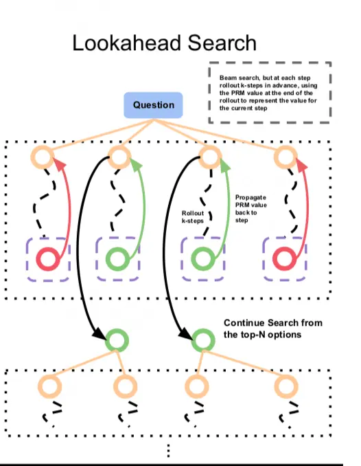
• For a problem, we first sample N steps 1 in parallel (e.g. N=4 in the above figure)

• At this point, we are not in a hurry to directly use PRM to rate step 1. For each step 1, we let it continue to generate K steps downwards . Then send the last steps to PRM for scoring, and select the top M results with the highest scores, returning their corresponding step 1. Now these step 1 are the final results we have selected.

• Starting from step 1, repeat the above steps until the set search stop condition is reached.

It is not difficult to see that the core of lookahead search is to first “look ahead K steps” when filtering each step, and use the benefits after K steps to evaluate the results of the current step. So, the beam seam can be seen as the K=1 version of the lookahead seam.

It is worth mentioning that if you have understood MCTS (Monte Carlo tree search algorithm) You will find that lookahead seam is very similar to it in a broad sense. In MCTS, when searching for the best path (strategy), we use some random factors during the search process to achieve multiple objectives Explore To estimate the value of each step and then learn the value function. In lookahead search+PRM, this trained and fixed PRM replaces the explore process in MCTS At this point, lookahead search only needs to be responsible Utilize (exploit) That’s enough. So, lookahead search + PRM， In a broad sense, it is a method of MCTS. We will explain MCTS in detail in the following article.

2.4 How to choose the best search method

There are so many search methods, how should we make choices to ensure the best search results? (That is, to optimize the inference performance of the model)

We can first guess intuitively what factors will affect the search performance of the model:

• Search for generation budget This refers to the sampling quantity N. How many parallel samples do you want to do when searching for a problem. The reason we consider N is that the computing power of GPUs is limited.

• Difficulty of the problem For simple questions, the model may be able to provide answers using pre trained knowledge without introducing complex search methods. For more difficult problems, it may be necessary to design a good search method to guide the model to think step by step.

Based on these two intuitive thoughts, the author conducted the following two sets of experiments:

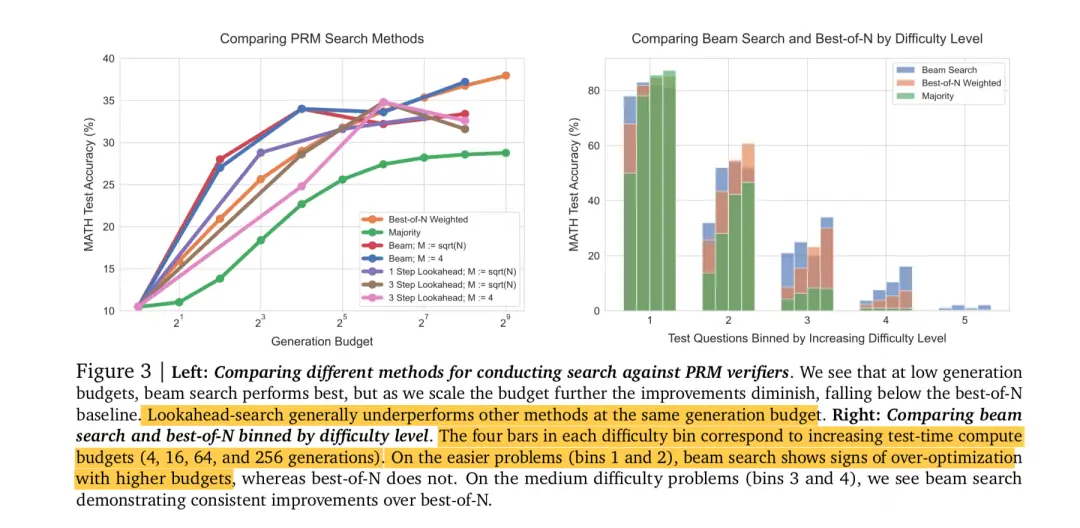
(1) The impact of search budget on search performance

Let’s first look at the left image, which explores the impact of search budget on the inference performance of the model . Orange represents best of N weighted, which is the baseline we use for comparison. From the figure, it can be seen that:

• When the search budget is small (i.e. parallel sampling N for a problem is small) ，beam seach > best-of-N > lookahead

• When the search budget is large (i.e. when the parallel sampling N for a problem is large) ，best-of-N > beam seach > lookahead，beam searchM，best-of-N

• The most complex lookahead search method performs at the bottom of the trend.

We can intuitively provide some explanations for the above phenomenon (The paper is also very vague here, so the author still made a subjective understanding based on some of the content of the paper):

• When N is small, it may be difficult to directly hit the best answer among N parallel sampled results for a problem . At this point, by using more complex search strategies such as beam search, shifting from one-time sampling to step-by-step careful selection, better results may be achieved. When N is large, the same can be inferred.

• stay If PRM is trained well enough, at each step of the search, we can focus more on utilizing the current (expand) rather than exploring the future (explore) As mentioned earlier, the essence of exploration is to find a better value function, but its risk is strong randomness. So the complex lookahead method does not perform well in our scenario.

(2) The impact of problem difficulty on search performance

I Let’s take a look at the image on the right again, which explores the impact of problem difficulty on search performance. Bin1 to Bin5 represent 5 levels of difficulty (from easy to difficult), and the 4 columns under each bin represent different search budgets (4, 16, 64, 256). Perhaps considering the poor performance of lookahead in previous experiments and the fact that beam search itself can also represent a type of lookahead search, the author directly removed lookahead from the experimental subjects. From this experiment, we can observe that:

• （3，4），beam search > best-of-N；

• （1，2），best-of-N > beam search（beam search）。

• On the most difficult problem (difficulty 5), both performed poorly.

• Of course, the above trends are only general, and the specific fluctuations are also limited by the search budget. You can take a closer look at the experimental chart on your own.

We can provide some intuitive explanations for the above phenomena (also including the author’s subjective interpretation):

• On simple questions, the knowledge acquired by the model during the pretrain phase has a high probability of providing the correct answer . That is to say, if you randomly sample N results for a simple question, there is a high probability that there will be a correct answer in these N. At this point, there is no need to introduce complex search methods (such as PRM) and conduct step-by-step evaluations. After all, the evaluation process is chain like, and if there is a step evaluation error, there may be a chain of negative effects. The same can be applied to complex problems.

• When the problem is particularly difficult, the post-processing mode of “PRM+some kind of search method” may no longer be applicable independently. At this time, it may be more necessary to improve the pre training knowledge of the model in the pretrain stage . This reminds me of openAI o1, which can also achieve good results in some complex mathematical reasoning. Therefore, although the official statement states that it has increased computing power in the inference stage (including post-processing methods of reinforcement learning), perhaps it has also processed the base model, such as increasing the proportion of code and mathematical logic knowledge. Or it is possible to change this ratio and retrain the base model directly.

(3) Summary of Search Methods

1. The effectiveness of search (i.e. the inference effect of the model) is limited by the search budget and the difficulty of the problem, and we choose the appropriate search method within these limitations.

2. When the search budget is small and the problem is difficult, the beam search method is more suitable, but attention should be paid to adjusting hyperparameters

3. When the search budget is large and the problem is simple, the best of N method is more suitable

4. When PRM is trained well enough, more complex search methods such as lookahead search may not perform well

5. When the problem is particularly difficult, the effectiveness of the test time scaling law may be limited, and it may be necessary to re-examine the pretrain stage by increasing/adjusting the data ratio, expanding the model size, and injecting more relevant knowledge into the pretrain model.

3、 Method 2: Directly changing the output distribution of the model

In the previous text, we introduced the pattern of using “PRM+search method” to guide the step-by-step reasoning process of the model and find the best answer. Now? Let’s take a look at another method to improve the accuracy of model inference: directly changing the output distribution of the model (refining the proposal distribution).

In the mode of “PRM+search method”, we have mentioned that training the model through SFT can generate results in a given format (step-by-step thinking). This step only serves as format alignment and is not responsible for the quality of the thinking process. that At this point, you must be thinking: If I could use data with high-quality thinking steps to directly model SFT, wouldn’t the same effect be achieved? And once such a model is trained, in the subsequent inference stage, it will autonomously start thinking step by step after encountering a problem, without the need for any search methods or PRM, just using its generation ability, as shown in the following figure:

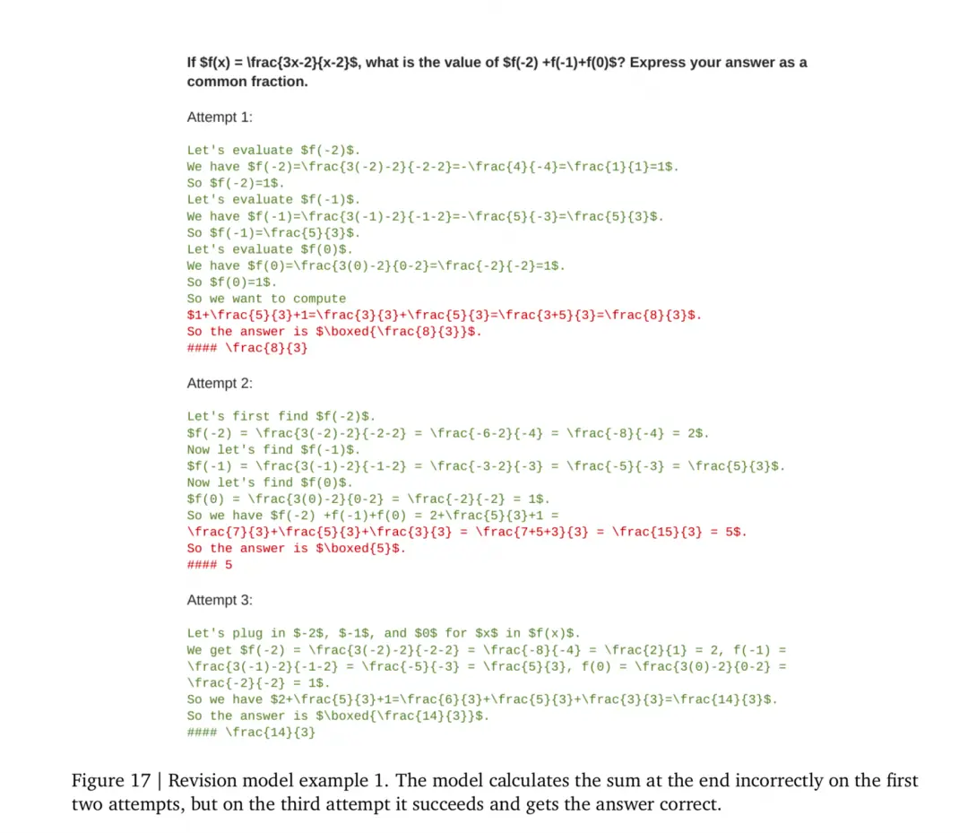
As shown in the above figure, after incorporating the problem, the model went through multiple iterations and gradually approached the correct result.

There is nothing to say about the process of training such a model in SFT, the key is in the aspect of “how to collect high-quality SFT data” So next, let’s take a detailed look at this point. In addition to the training method provided in this article, the two models STaR and Quiet STaR that we have recently seen frequently in the openAI o1 hot search can also be roughly classified into this category (Quiet STaR has some special features and covers more clever ideas). In the following articles, we will combine the source code to take a look at these two interesting models.

3.1 Collecting SFT data

How can we generate high-quality SFT data that covers intermediate thinking steps with minimal cost? Let’s take a direct look at the authors’ approach:

• Firstly, we have supervised data such as’ question+answer ’, but we lack an intermediate process. We hope that the model can simulate human thinking and gradually approach the correct answer by trying various attempts.

• Then, using the same method, we first fine tune the format of the model to produce “intermediate results+answers” (note that it is not multiple attempts as shown in the above figure, but a single attempt). This step is only responsible for the format and not for the quality

• Next, using the model, for each question, N attempts are sampled in parallel (single attempt=intermediate result+answer, N=64), and some attempts that contain invalid answers are also filtered out (review again, invalid!=error)

• Since each attempt contains an answer, which is labeled, we can know which attempts gave the correct answer. We say these attempts are correct.

• Now, we hope to match each correct attempt with several incorrect attempts as training data. That is to say, our training data is in the form of “problem+several incorrect attempts+correct attempts”. This step is to let the model simulate the human thinking pattern and deduce the correct attempt from the incorrect attempts step by step. The specific method is as follows ：

• Uniformly sample a number from 0 to 4, denoted as x. Now for each correct answer, we need to match it with x incorrect answers

• First, from all the incorrect answers, find the one that is most similar to the correct answer based on the editing distance (editing distance may not be a good way to accurately measure similarity, but it is sufficient for this scenario)

• Then randomly sample x-1 from the remaining incorrect answers.

• For a correct answer, we can now proceed according to (Question, randomly incorrect answer x-1, most similar incorrect answer, correct answer) To form an empirical data, this data is called trajectory We will use it to perform SFT on the model. The correct answer is the part that the model needs to predict, The reason for choosing a relatively similar incorrect answer here is to let the model know that it is constantly correcting its mistakes and learning better 。

• ，，x < 4，0～x，。 This is done to ensure that our trajectories cover as many different numbers of incorrect correct answer combinations as possible.

When you examine the method of collecting SFT data above, you may feel that there are many areas for improvement, such as: Just because the answer is correct, does that mean the attempt is correct? There may be errors in its intermediate steps, which could be a false positive . So, one possible improvement approach is to still introduce the trained PRM and evaluate the intermediate steps, which is more conducive to selecting the most correct attempts as much as possible. This example is given to illustrate that this article only provides a possible data collection method, not a data collection standard. In our actual research, there are still many areas that can be explored, but their core is the automated collection of supervised data.

3.2 Stop time for model training

Let’s take another interesting question: When we use the above data and enter SFT training, how should we determine the time when SFT training can be stopped?

• The loss of the model on the evaluation set determines the training level of the model. We certainly expect the loss of the evaluation set to gradually decrease. When we observe an increase in the loss of the evaluation set, it often means that the model has begun to overfit. We usually stop training the model early before this trend begins.

• However, in this experiment, the author observed that even after the evaluation set loss increased for a long time, the model still performed very well. This is because the evaluation set data is off policy, and the model is constantly updating. The distribution of the evaluation set data can no longer keep up with the model, so the loss of the model on it cannot truly reflect the training situation of the model

• So, in the end, the author chose to stop training the model after discovering the overfitting phenomenon for a period of time

3.3 How to choose the best generation method

Normally, if such an SFT model is trained well enough, then we feed it a problem and just need to let it continuously generate attempts until <end> Then take the last attempt. However, in reality, there may be the following issues:

• We cannot guarantee that the last attempt will always be correct. It is highly likely that the correct attempt was generated in the middle, but the model corrected it again.

• We cannot guarantee that for a question, only one answer will be generated (i.e. one attempts chain), and there will always be the correct attempts.

So, although theoretically we can use the SFT model. But in order to achieve better results, we will still use the “verifier+search method” approach for inference . The reason why it is written as’ verifier ‘instead of’ PRM ‘is that’ verifier ‘may not necessarily be based on processes, but can also be based on results (orm). Let’s take a look at an architecture diagram:

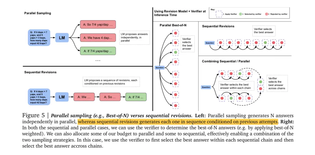
• [Left side parallel sampling]: This only tells us how parallel sampling is done, and does not tell us which result to choose. In our scenario, parallel sampling represents generating multiple attempts chains for a single answer (each chain containing several attempts)

• [Left side sequential revisions]: This is the most naive way of reasoning and also generates a single attempt chain that contains multiple attempts. Only explain the process, without discussing the selection plan

• [Right side planar best-of-N]: The figure on the right begins to explain the selection scheme. We have introduced a verifier for selection here. For a problem, the model can sample multiple results in parallel, each of which is a series of attempts chains, and finally use a verifier to select the highest scoring attempts chain.

• [Right side sequential revisions]: Similarly, by introducing a verifier, we have the model generate multiple instances in order, but we cannot fully believe that the last instance is necessarily correct. So we use a verifier to help us determine which attempt to choose in this chain.

• [Right side combining sequential/parallel]: Generate multiple chains simultaneously, with several instances in each chain. First, use a verifier within each chain to find the best attempt, then put all the best attempts together and use the verifier to find the optimal one

The author also uses experimental methods here to determine which generation method to use, subject to the limitations of search budget (number of samples N) and problem difficulty. We won’t include the experimental content anymore. Everyone can read the article on their own, and here we will directly give the conclusion:

1. On simple problems, using sequential generation (finding the best attempt in a single attempt chain) yields better results

2. In complex problems, combining sequential and parallel methods yields better results, but it is important to choose appropriate hyperparameters

4、 Pretrain or Inference?

In the above process, we introduced two methods of concentrating computing power on the inference/post training stage to improve the final inference performance of the model (but as mentioned in the introduction of this article, these are actually two frameworks, and the specific approach refers to examples. In practice, we can make many variations). Given your understanding of these methods, you must be eager to learn from the quantitative experimental results: how much better can the results under the guidance of inference scaling law be than those under the guidance of pretraining scaling law? In other words, if I allocate the same computing power to inference and pretrain, how will their performance be?

In the paper, the author briefly provides some modeling indicators and explanations. The author has attempted to understand them from a more detailed perspective, but unfortunately, there are many ambiguities and ambiguities in the description provided in the paper, and with my current ability, I am unable to provide a consistent explanation. So in this section, the author plans to directly release the experimental effect diagram to explain the problem of pretrain vs inference intuitively:

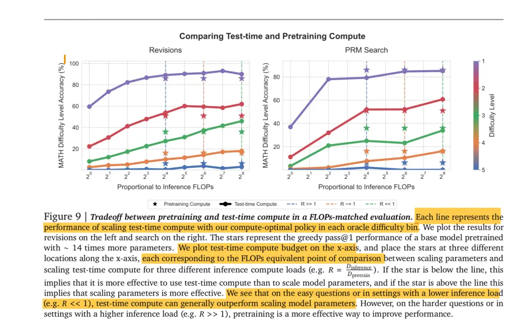
The left and right images show the effects of using PRM guided search and directly changing the model output distribution, respectively. The experimental methods for both are consistent, so we only need to look at one of the images. In this experiment:

• The horizontal axis represents computing power (FLOPs)

• The vertical axis represents the inference performance of the model.

• Different colored curves represent different levels of difficulty in solving problems

• The curve with dots represents the effect of the model when all the computing power is used for inference

• Each dashed line represents the exchange ratio of computing power between pretrain and inference. The asterisk indicates the final inference performance of the model when a certain proportion of computing power is given to the pretrain (it cannot be completely switched to pretrain, as the pretrain stage also requires computing power for inference after continuing training)