Modern LLM Basic Technology Compilation

Author: hadiii， I am currently pursuing a Master’s degree in Electronic Information at Peking University

Original text: https://zhuanlan.zhihu.com/p/713794852

Before 0 starts

This article starts from the Llama 3 report and summarizes some modern LLM techniques Basic “means that it is not too detailed about some specific details, but rather hopes to obtain a relatively comprehensive article that includes pre training, post training, inference, and can introduce specific technologies such as RM, DPO, KV Cache, GQA, PagedAttention, Data Parallelism, and so on. Due to the large amount of content and the inability to provide detailed information, it is recommended that everyone reorganize it into their own notes.

The main reference of this article is the original report of The Llama 3 Her of Models by Llama Team, as well as the intensive reading series of newly published papers on Mu Shen’s return to Bilibili. It also includes some excellent articles by Zhihu.

1 Intro

Illustration of the overall architecture and training of Llama 3

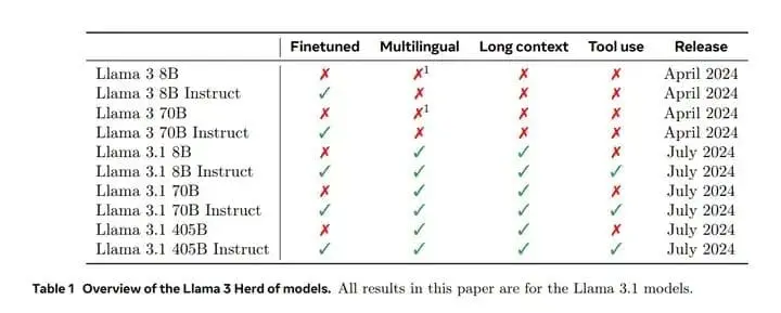
Overview of the Llama 3 Herd of models.

1.1 The main stages of modern basic model training

（a） Pre training stage (Pre training stage): The algorithm is relatively straightforward, usually using a large amount of data to make next word predictions.

（b） Post training stage (Post training stage): The algorithm is relatively rich, including SFT, RLHF, DPO, and so on. In terms of tasks, this includes having the model perform instruction following tasks, aligning model preferences with human preferences, or improving the model’s ability to perform specific tasks such as code, math, roleplay, and so on.

From past models, it can be basically assumed that GPT1, 2, and 3 are all doing pre training, while InstructGPT and RLHF are doing post training. The above is a relatively general introduction.

1.2 Key to Modern Basic Model Training

Meta：We believe there are three key levers in the development of high-quality foundation models: data, scale, and managing complexity.

Meta believes that the key to modern basic model training is: data, scale, and managing complexity。

（a） Regarding data The Llama series has a tradition of stacking data: compared to Llama 2’s 1.8T pre training corpus, Llama 3’s pre training corpus is stacked into 15T multilingual tokens.

Mu Shen: 15 T may be the approximate upper limit of text data that can be captured on public networks at present. This’ upper limit ‘means that instead of looking for incremental data, it is better to adjust the quality of existing data.

（b） Regarding Scale Llama 3.1 offers three scales: 8B, 70B, and 405B. The performance differences of each scale can refer to the benchmark below.

（c） Regarding management complexity Complexity management, in other words, the Llama 3 algorithm is relatively simple. Llama 3 chose a standard dense Transformer model architecture with only minor adjustments, without selecting MOE. In terms of post training, Llama 3 adopts SFT, RS, and DPO, a relatively simple process, rather than the more complex RLHF algorithm, which often has poorer stability and is more difficult to scale. These are all design choices. Chapters 2 and 3 will provide a detailed introduction to the relevant technologies.

1.3 Benchmark Performance

The benchmark performance of each specification model of Llama 3 is as follows. Briefly introduce MMLU and IFEval among them.

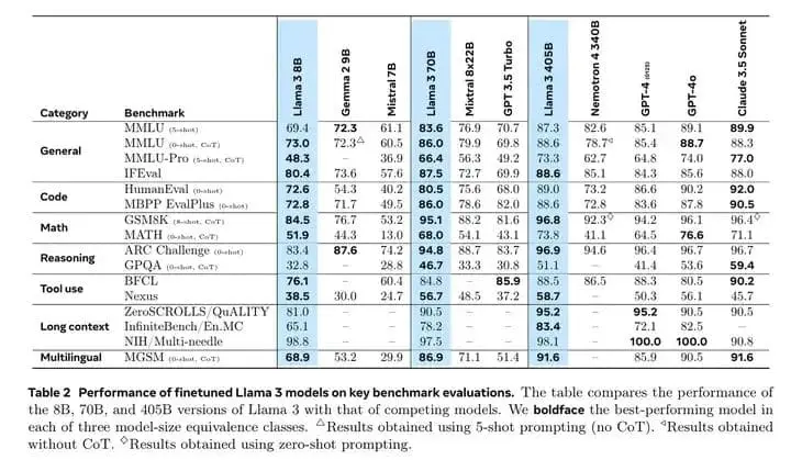
Performance of finetuned Llama 3 models on key benchmark evaluations.

(a) MMLU series Similar to multiple-choice questions in various exams, it mainly tests the knowledge aspect of the model (memorizing answers).

Question: Glucose is transported into the muscle cell:Choices:
A. via protein transporters called GLUT4.
B. only in the presence of insulin.
C. via hexokinase.
D. via monocarbylic acid transporters.Correct answer: A

The original MMLU is a relatively old benchmark, and there is a possibility of overfitting for everyone. MMLU Pro is relatively updated, and it can be seen that there is a significant difference between 8B, 70B, and 405B on MMLU Pro, indicating that the parameter size and the amount of knowledge internalized into the weights are still highly correlated.

（b）IFEvalIF stands for Instruction Following, which tests the model’s ability to understand and follow instructions. The original text can be found at:IFEval Dataset | Papers With Code[1]。

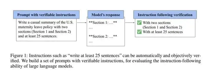
IFEval Example

On IFEVAL, the difference between 8B and 70B is still significant (80.4/87.5), while the difference between 70B and 405B is no longer significant (87.5/88.6). After the parameter scale reaches a certain level, it may gradually become insignificant to increase the IF capability by expanding the scale.

(c) The remaining benchmarks They are slightly vertical and contain Code, Math，Reasoning，Tool use，Long context，Multilingual， Please refer to the original report.

Addendum: Since the above evaluation sets all have the risks of overfit and leakage, are there any other benchmarks? Of course, for example, benchmarks like LiveBench that update monthly,LiveBench[2]. However, there is no perfect benchmark in the world, especially for specific businesses.

Overall, there are still significant differences between 8B and 70B in various aspects, but the differences between 70B and 405B are relatively small in the above evaluation clusters. The inference and training of 405B are relatively slow, and in general, 70B is the preferred choice for complex applications. If it is particularly complex, then consider 405B, as the cost-effectiveness will still be slightly lower. It is worth mentioning that Llama 3.1 70B is close to the level of Claude 3.5 sonnet on IFEval.

2 Pre-Training

Meta：Language model pre-training involves: (1) the curation and filtering of a large-scale training corpus, (2) the development of a model architecture and corresponding scaling laws for determining model size, (3) the development of techniques for efficient pre-training at large scale, and (4) the development of a pre-training recipe. We present each of these components separately below.

The previous text provided a general explanation of the key points of Pre Training.

2.1 Pre-Training Data

• • Web Data Curation

The key points of pre training data processing include de duplication methods and data cleaning mechanisms, namely deduplication and cleaning. If not done well, the quality will be poor. The Web Data Curtation section in the specific report mentions the following content:

（a）PII and safety filteringThe report mentioned that domain names containing PII (personally identifiable information) and adult content were removed from the pre training data. But there is no specific standard to anchor whether the data belongs to PII and adult content, and no example is given, so it is likely that some are mixed in.

（b）Text extraction and cleaningSince web data is raw HTML content, Llama built a parser to parse various types of documents. An interesting point is that the report believes that Markdown is harmful to the performance of the model, so all Markdown markers have been removed. But there is no explanation on how to do it after removing it.

（c）De-duplicationLlama used three levels of deduplication, URL，document, and line level。 Specifically, URL deduplication means retaining the latest version of the page corresponding to each URL. At the document level, global MinHash is used to remove approximately duplicate documents across the entire dataset. The specific approach at the line level is to search every 30M of documents and remove text lines that appear more than 6 times.

（d）Heuristic filteringHeuristic filtering. Including filtering of n-grams, if n is long and there are many repetitions, the line will be removed. A typical example is logging text. This also includes filtering out dangerous words. If a webpage contains too many dirty words, they will be removed. The report also mentioned the use of a method based on token distribution Kullback Leibler divergence (KL divergence) to filter out overly bizarre data. If the distance difference between a document and other documents in KL calculation is too far, mark the document as a strange document and remove it.

The concept of KL divergence is commonly used to measure the degree of difference between two probability distributions. Defined as:

（e）Model-based quality filteringModel based classification. For example, fasttext and Roberta based classifiers trained on Llama 2 can be used for classification, including high quality or low quality, as well as domain tagging and so on.

（f）Code and reasoning data and Multilingual dataIt is also a pipeline for extracting specific data, which involves spending money and manpower to do some work.

• •  Data Mix

Data matching is indeed quite important, and it is a highly experimental task (alchemy) that burns money and time to produce results. The report mentioned some experiments on knowledge classification and scaling law.

**（a）Knowledge classification.**Using a classifier to classify data into categories such as objective knowledge, entertainment gossip, adult content, etc Entertainment gossip data is not very good for the model, but after classification, this type of data can be reduced.

**（b）Scaling laws for data mix. ** Conduct experiments with different ratios to observe changes in indicators. To be more specific, it is to conduct different proportioning experiments on different small models and then use them to predict the optimal proportioning on a larger scale.

In summary, the final pre training data consists of approximately 50% general knowledge, 25% mathematical and reasoning data, 17% code data, and 8% multilingual data.

• •  Annealing Data

The report found that annealing the learning rate on a small amount of high-quality code and math data can improve the benchmark performance of pre trained models. This is very intuitive, that is, ‘memorizing more questions before the exam will lead to better results’. （？）

Specifically, after training with a large amount of general data, a small amount of high-quality domain specific data is used to continue training while gradually reducing the learning rate. Llama 3 adopted the method of linearly annealing LR to 0 in the last 40M token of pre training, while adjusting the data ratio accordingly. Finally, the 8B model showed good performance on the GSM8k and MATH validation sets, but the improvement on the 405B model was negligible, indicating that models with this parameter size may not require specific in domain training samples to improve performance.

Meanwhile, the report mentions that annealing can be used to evaluate the quality of domain specific small datasets, which is more efficient than conducting relevant experiments using Scaling Law.

2.2 Model Architecture

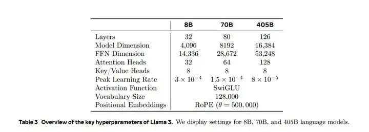
Overall, Llama 3 has made the following changes compared to 2: GQA, attention mask for different documents within a sequence, vocabulary for 128K tokens, and adjustments to RoPE.

• •  ** -> KV Cache -> GQA**

Llama 3 uses the standard Dense Transformer architecture, and the performance improvement mainly comes from the improvement of data quality and diversity, as well as the increase in training scale (to be honest). Of course, there are some changes compared to Llama 2:

For example, the Grouped Query Attention: GQA mentioned above is used to accelerate inference and save decoding memory. For models of 70B and above, it is almost a necessary technique. GQA involves KV Cache, which involves the basic reasoning process, so start writing from reasoning.

(a) Basic reasoning process

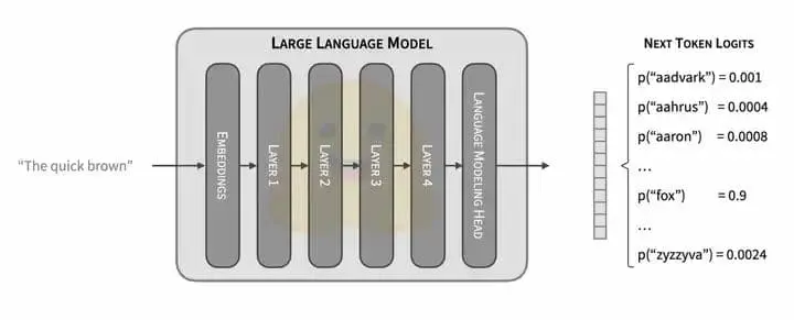
LLM reasoning process

1. The input text is divided into n token/token ids according to the vocabulary, and the n token ids are mapped into n embedding vectors, that is, 1 embedding matrix;

2. The embedding matrix is passed through L transformer blocks (with various attention calculations and FFN layers inside), and in the last layer, an embedding matrix with the same shape as the input is output;

3. The output of n embeddings is passed through a linear layer lm-head, whose output shape is consistent with the size of the vocabulary. Adding another softmax to the output of the linear layer yields the probability score of the next token;

4. Then sample according to the decoding strategy. After the Next token is calculated, the input token sequence (length n+1) is added to continue calculating the n+2nd token, which is called autoregression.

（b）KV Cache

Since the intermediate results of the L Transformer blocks can be saved when calculating the n+1th token, they may be reused. We willLayer, layerThe output of a token is denoted as. It is not difficult to find that when calculating the n+2nd token, a large part of the intermediate results are the same as when calculating n+1. It can be expressed as:

Enter token sequence:The input token sequence isConsistent, so we use caching to reduce a significant amount of computation.

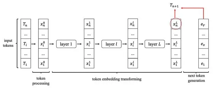
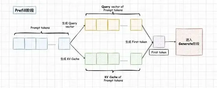
Therefore, the LLM inference process is divided into two stages: Prefill and Decode. The Prefill stage performs parallel calculations on all tokens in the Prompt to obtain the KV Cache of all tokens in the Prompt and calculate the first token. The KV Cache calculated from Prompt Tokens will be saved for reuse in the Decoding stage;

The decode stage is an autoregressive process where, for each new token decoded, all previously calculated KV caches are used to calculate the Attention of the current query token. Therefore, when the output length becomes larger or the context is long, KV Cache will occupy a large amount of video memory.

This paragraph and the following image are referenced from: [KV Cache Optimization] MQA/GQA/YOCO/CLA/MLKV Notes: Intra layer and Inter layer KV Cache Sharing[3] 。

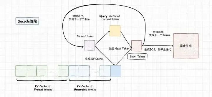
So now there is also the concept of prefix caching, which simply means caching the KV cache of a specific prefix for future use. It is very effective for tasks with complex instructions, long prompts, or multi round dialogue scenarios. VLLM can easily enable prefix caching and optimize fixed tasks with long input and short output. KV Cache has a wide range of directions to explore and is one of the core areas of LLM inference optimization.

（c）GQA，Grouped Query Attention

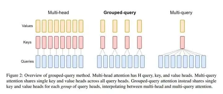
GQA is one of the methods to reduce the size of KV Cache at the model level. The convention before discussing GQA was to talk about MHA and MQA.

MHA， Multi Head Attention, also known as Multi Head Attention, is the attention form in the original Transformer text. As shown in the figure below, each Query vector in MHA corresponds to a Key, Value, and its output concatenates the outputs of each attention head. Therefore, there will also be more KV Cache stored.

MQA， That is, Multi Query Attention. As shown in the figure below, MQA’s approach is quite straightforward, which is to share one KV for each attention head. Obviously, compared to MHA, the KV Cache usage is directly reduced to 1/head_num. However, due to structural modifications and a decrease in the number of parameters in the Attention section, the model’s performance is inevitably affected. MQA seems to be somewhat violent.

Therefore, a balanced version emerged, namely GQA, Grouped Query Attention。 Consistent with the figure, the queries are grouped with each corresponding KV, and a compromise method is used to reduce computational complexity and KV Cache size.

• •  RoPE， Rotation position encoding

Firstly, we should talk about the classic sine encoding. As mentioned in the previous inference process of LM, tokens are mapped to embedding vectors. In the structure of classical transformers, this embedding vector is the superposition of word embedding vectors (the ‘isolated’ semantics of entities) and positional encoding (the ‘associated’ semantics between entities). How to characterize the location of a token is a problem of location encoding research.

Hands on Deep Learning PyTorch Edition: Key Notes[4] The position encoding of the classic transformer architecture is sinusoidal encoding.

There may be some issues with sine encoding, such as weak representation of relative positions. RoPE is attempting to address these issues.

2.3 Scaling Laws

The initial form

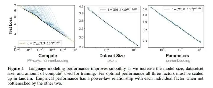
Simply put, it means that some experimental results from small models can be used to predict the results of larger models. Scaling Law was proposed by OpenAI and has two well-known conclusions:

1. For decoder only LM, computational complexityModel parameter quantity, data sizeAll three are satisfied. Among themThe unit is FlopsIs the number of tokens;

2. The final performance of the model mainly depends onRelated, with low correlation to the specific structure of the model (height, short, fat, thin).

-**What is the content of the Llama report**

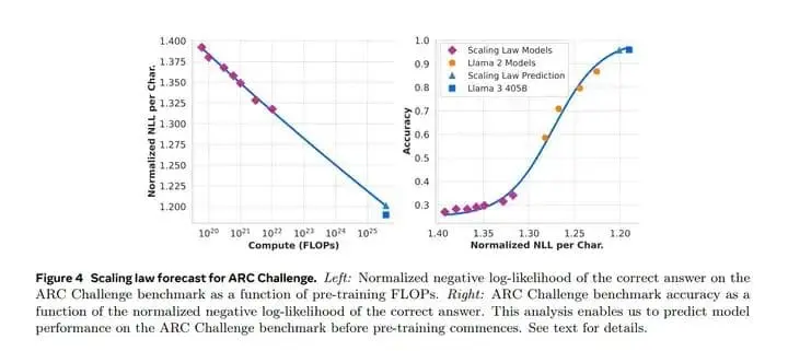
The previous Scaling Law prediction method mainly started from the next token prediction loss (validation loss during training), but this loss may not be absolutely correlated with specific task performance. Because the next token prediction loss is not absolutely linked to specific task performance (such as mathematics). So Llama 3 used a two-stage method when conducting the Scaling Law experiment:

Step 1: Predict the NLL loss of the model on specific downstream tasks, which is still linked to compute (FLOPs) and forms a functional relationship;

Step 2: Use Scaling Law to associate the loss in Step 1 with the specific task accuracy. For example, an NLL loss of 1.4 corresponds to an accuracy of 0.25, and an error of 1.2 corresponds to an accuracy of 0.95. Therefore, this rule can also be decoupled from the actual situation, resulting in a Scaling Law curve for a specific benchmark, with loss and accuracy on the x and y axes, respectively.

Please refer to the following figure for details. The ARC Challenge benchmark is a multiple-choice task set for reasoning. The prediction of Scaling Law is quite accurate. However, it should be noted that the benchmark curves for different tasks may also vary in length.

2.4 Training Recipe

The pre training strategy of Llama 3 mainly consists of three steps, namely: (1) initial pre training, (2) long context pre training, and (3) annealing

Initial Pre-Training

Mainly some details. Translate it simply. We pre trained Llama 3 405B using AdamW, with a peak learning rate ofThe linear warm up is 8000 steps, and the cosine learning rate is expected to decay to 1200000 steps）. In order to improve training stability, we used smaller batch sizes in the early stages of training and subsequently increased batch sizes to improve efficiency. Specifically, we used an initial batch size of 4M tokens and a sequence length of 4096. After training 252M tokens, we doubled these values to obtain 8M sequences of 8192 tokens. After training 2.87 T tokens, it will be doubled again to 16M. We found that this training formula is very stable: we observed very few loss spikes and no intervention is needed to correct the bias in model training.

We also made some adjustments to the data mix. For example, gather more non English data, mathematical data, and the latest online data.

Long Context Pre-Training

Translate it simply. In the final stage of pre training, we train long sequences to support context windows for up to 128K tokens. We did not train long sequences before because the computational complexity in self attention layers increases with the square of sequence length. We gradually increase the supported context length and perform pre training until the model successfully adapts to the increased context length.

We evaluate the successful adaptability through the following two points: (1) whether the performance of the model in short context evaluations has been fully restored, specifically in the MMLU evaluation sets; (2) Can the model perfectly solve the ‘needle in a haystack’ task with a length reaching this value.

In the pre training of Llama 3 405B, we gradually increased the context length in six stages, starting from an initial 8K context window and eventually reaching a 128K context window. This long context pre training phase used approximately 0.8T tokens.

Annealing

Refer to section 2.1 Pre Annealing Data for the same content as Annealing Data.

3 Post-Training

The following figure clearly summarizes the post training approach of Llama 3, which includes elements such as RM, SFT, RS, and DPO. This chapter will introduce them one by one. Post training is what the vast majority of NLPs in the industry do.

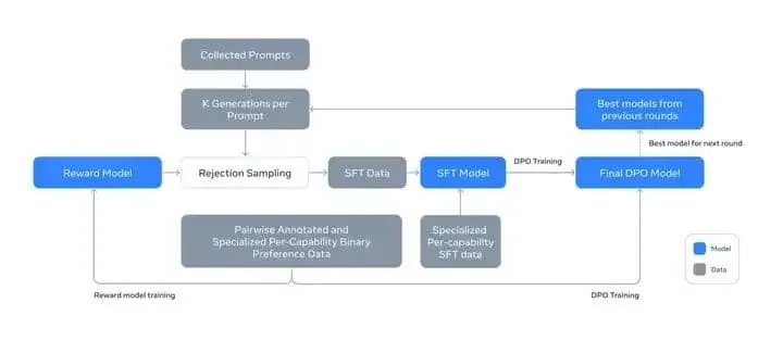
Illustration of the overall post-training approach for Llama 3.

The backbone of Llama 3’s post training strategy is a Reward Model and a Language Model. Firstly, using preference data annotated by humans, train an RM on a pre trained checkpoint. Then, perform SFT on the pre trained checkpoint, align it with DPO as the best model for this round, and proceed to the next iteration to participate in the Rejection Sampling process.

Note that the training is iterative, meaning there are multiple rounds of training with the same method. Specifically, Llama 3 underwent 6 cycles. Collect new preference labels and SFT data in each cycle, and sample synthesized data from the latest model.

3.1 Reward Model

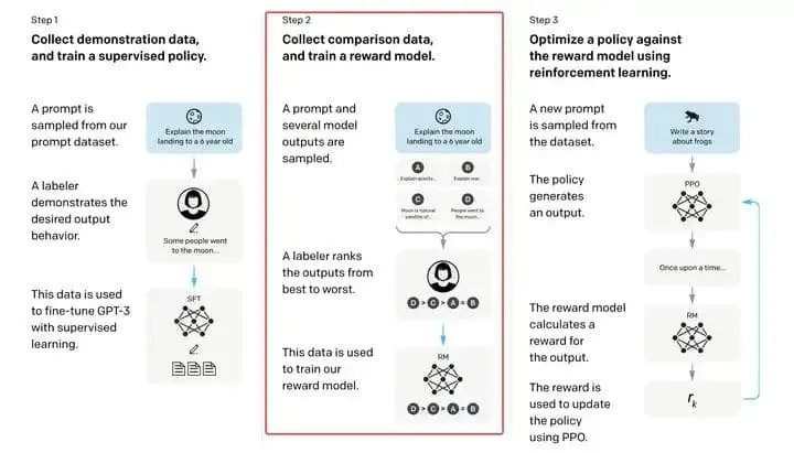
The red box represents the training path of RM

Reward Model（RM）。Reward Model”“（A >> B > C = D），（，，）。，。

，A > BA > B，，，（margin loss），Llama 2 Part of:

Preference Data Construction

Llama provided a detailed explanation of the construction process of Preference Data. Here are a few steps:

**step 1.**Train multiple models for annotation using different data ratios and training strategies. Deploy multiple different models and sample two responses from different models for a specific user prompt.

**step 2.**Students will rate the responses based on the standard of “significantly better”, which includes four levels: significantly better, better, slightly better, or marginally better。

**step 3.**After the preference annotation is done, encourage the annotators to “edit” the chosen response, that is, they have already chosen the better answer in the previous step and made better changes. You can either directly modify the chosen response itself or modify the prompt to refine these data.

，ranked response，edited > chosen > rejected。，。

train

Training is similar to Llama 2. However, Llama 3 actually removed the margin loss from the loss function, as mentioned earlierBecause it has been observed that the improvement effect of margin gradually weakens as the data scale expands, it is better to simplify.

3.2 SFT

SFT is probably the first choice for most students to engage in LLM training. SFT， The process of training target tokens involves using standard cross entropy loss and mask prompt loss.

SFT Data Construction

There are many sources for SFT data: data from Rejection Sampling, synthetic data tailored to specific abilities, and a small amount of manually annotated data.

Rejection Sampling

The process of rejection sampling involves fixing the model and prompt, allowing LM to sample K different answers, and selecting the optimal answer based on RM’s K different scores. Then use the optimal answer as SFT data for iterative training. Among them, the model is usually the best performing checkpoint in the previous round of training, and K can be adjusted, usually between 10-30. Sampling also involves many details, including the construction of preference pairs. For example, rejected may not be able to brainlessly select the worst, which requires experimentation.

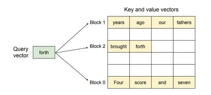
In order to improve the efficiency of rejecting sampling, Llama 3 adopts PagedAttention. In PagedAttention, memory waste only occurs in the last block of the sequence, which can effectively improve throughput. The memory sharing of PagedAttention is also well optimized. In Rejection Sampling, multiple responses are generated by the same prompt. In this case, the computation and memory of the prompt can be shared in the output sequence. Here are some brief introductions.

PagedAttention

think of blocks as pages, tokens as bytes and requests as processes。

PagedAttention is also a popular choice for the vLLM inference acceleration framework. Everyone should have taken OS courses and understood the concepts of virtual memory, memory paging management, and memory fragmentation. PagedAttention is also inspired by OS, which believes that KV Cache does not need to be stored in continuous memory, but rather introduces the concept of blocks as “page”, bytes as “token”, and processes as “request”, just like the operating system.

In Section 2.2, we mentioned that since the intermediate results of the L Transformer blocks can be saved when calculating the n+1th token, they may be reused. This is called KV Cache.

But KV Cache is very large and requires a contiguous memory to store. Moreover, we do not know how much contiguous memory needs to be reserved before receiving the sequence, so we can only allocate a cache of the maximum possible length in advance, resulting in a lot of waste, which is called “internal fragmentation”. However, due to the allocation of memory for multiple sequences, the remaining memory is not sufficient to allocate to new sequences, and this part of memory is actually useless, resulting in waste, which is called “external fragmentation”.

PagedAttention allows storing consecutive keys and values in non contiguous memory space. Specifically, it divides the KV cache of each sequence into blocks, each block containing a fixed number of token keys and values. Therefore, for one sequence, there will be at most one page with memory fragments. Due to block allocation, external fragments are completely eliminated. This is consistent with the problem solved by paging storage in the OS.

Returning to SFT Data, we finally obtained this data composition.

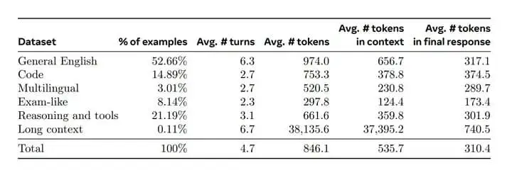
In terms of training details, when Llama 3 fine tunes 405B, the learning rate is 10 ⁻⁵, and the training steps are between 8.5K and 9K.

3.3 Rejection Sampling

Refer to Rejection Sampling in section 3.2 SFT.

3.4 Direct Preference Optimization

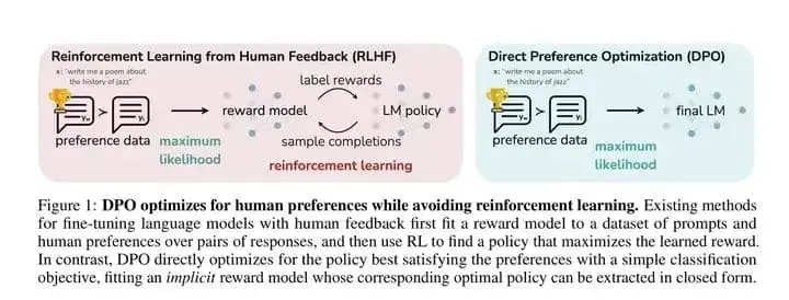
DPO is performed after SFT with the aim of aligning human preferences. DPO is a simplification of RLHF, aimed at bypassing complex RM training and other processes. RLHF first trains RM with annotated preference data and then guides the RL process, while DPO combines the losses of the two steps mentioned above.

Therefore, the training data for DPO is also human preference data, with a format similar to select rejected pairs. The losses of DPO are as follows

   #Data format of DPO
{    
    'prompt': '',
    'chosen': '',
    'rejected': ''
}   

DPO training details

During the training process, Llama 3 mainly uses the latest batch of preference data, which is collected through the best performing models in the previous rounds of alignment and requires RM. The advantage is that these data better fit the distribution of the Policy Model being optimized in each round. So this DPO is also iterative and belongs to on policy.

(a) The first detail Yes, due to the characteristics of the DPO loss function, if there are some common tokens in the chosen response and rejected response, it will lead to conflicting learning objectives, as the model needs to simultaneously increase and decrease the probability of generating these tokens. So Llama 3 masked the loss of formatting tokens, and the experiment found that if these tokens were counted as loss, it could lead to tail repetition and sudden generation termination of tokens.

(b) The second detail Yes, Llama 3 added a negative log Likelihood (NLL) loss to the chosen sequence. From the difference between NLL loss and standard cross entropy loss, we can simply understand NLL loss as SFT loss:

The benefit of adding NLL loss is to prevent the log probability of choke response from decreasing. The downside is that if the chosen response itself is not good enough, adding this SFT loss may not be very good, and specific analysis is needed for each problem.

3.5 Data Processing and Quality Control

Data quality is always the most critical. Due to the fact that most of the training data for Llama 3 is generated by the model, careful cleaning and quality control are required. This is consistent with the vast majority of vertical business models.

Data cleaning

Firstly, there are often some undesirable patterns in the data, such as the excessive use of emoticons or exclamation marks in Llama 3. Some very classic AI language styles also need to be noted, such as the tone issue of “too fond of sliding and kneeling”, and “I’m sorry” or “I apologize” when faced with problems. Such samples should not be too many in the dataset.

Data Pruning

Llama 3 also applies some model-based techniques to remove low-quality training samples to improve the overall performance of the model:

1. Topic classification Firstly, fine tune a small model (such as Llama 3 8B) to become a topic classifier, such as using a large amount of task data specifically for classifying text to perform SFT. Then classify all training data into coarse-grained categories (such as “mathematical reasoning”) and fine-grained categories (such as “geometry and trigonometry”).

2. Quality scoring Use Reward model and Llama based signal to score the quality of each sample. For RM based scoring, we consider data with scores in the top quarter of the RM score as high-quality data. For Llama based scoring, some scoring prompts were designed in Llama 3. Generally, English data is scored using three dimensions (accuracy, instruction adherence, and tone/expression), while coding data is scored using two dimensions (error recognition and user intent), and the sample with the highest score is considered high-quality data.

Finally, it was found that the divergence rate between RM score and Llama score was high, but it was found that combining these two mechanisms could achieve the best recall rate in the meta internal test set. Finally, select the samples marked as high-quality by the RM OR Llama 3 classification model.

3. Difficulty scoring Due to the desire to prioritize processing more complex samples for the model, the report mentions two difficulty assessment methods for scoring the data: Instag and Llama based scoring. For Instag, we suggest that Llama 3 70B annotate SFT prompts with intent, and the more intent, the higher the complexity. Based on the idea of Llama and similar to Quality scoring, some prompts were given to Llama 3 to score based on three dimensions.

4. Semantic deduplication Finally, perform semantic deduplication. Llama 3 first uses RoBERTa to cluster complete conversations, and then sorts them within each cluster by quality score x difficulty score. Next, traverse all sorted samples for greedy selection, retaining only samples with cosine similarity less than the threshold with the already seen samples in the current cluster.

4 Inference

Firstly, please refer to the content on the basic inference process, KV Cache, and GQA in 2.2 Model Architecture, and also refer to the introduction on PagedAttention in 3.2 SFT.

4.1 Parallelism

Parallelism, a part of LLM distributed training inference, including Data Parallelism and Model Parallelism, will be introduced in this section. It also involves some concepts of OS.

Data Parallelism

Data Parallelism， Data parallelism, where different input data batches (also known as mini batches) are independently received on each device and forward propagated to calculate the loss on that batch. During backpropagation, each device calculates gradients and exchanges these gradients with all other devices. Then, the average of these gradients is used to update the model weights on each device, ensuring that all devices have the same model weights at the beginning of the next training step.

The advantage is that it accelerates the training speed of the batch and can accommodate larger batch sizes of data. The downside is that each card also uses complete model weights, ensuring that a single card can fit in.

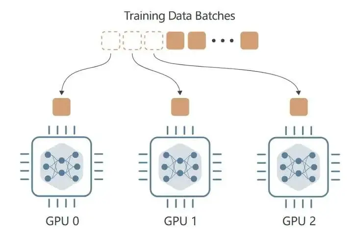
Data Parallelism

Model Parallelism

Model Parallelism。 Model parallelism, including Tensor Parallelism and Pipeline Parallelism. Model Parallelism solves the problem of not being able to fit a complete model weight on a single card, as each graphics card only contains some parameters. Generally speaking, parameters are divided according to layers, which is commonly referred to as Pipeline Parallelism. If none of the layers in the model can fit, splitting and training within the same layer is called Tensor Parallelism.

The advantage is that it can accommodate larger weights, but the disadvantage is that the cards in the later layers need to wait for the calculation results of the previous layers, so the GPU will have idle state. The same applies to backpropagation, where the cards in the front layer have to wait for the cards in the back layer.

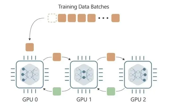
Pipeline Parallelism in Llama 3

When using BF16 values to represent model parameters, the Llama 3 405B model cannot be fully loaded into GPU memory on a single machine equipped with 8 Nvidia H100 GPUs. To solve this problem, the Llama 3 team used 16 GPUs on two machines (nodes) to perform BF16 precision model inference in parallel.

Within each node, utilize the high bandwidth of NVLink to enable tensor parallelism. Between nodes, the bandwidth of the connection is low and the latency is high, so pipeline parallelism (Gpipe) is used.

When using pipeline parallelism for training, bubbles are a major efficiency issue (see Gpipe paper for details). However, in the process of reasoning, this is not a problem as reasoning does not involve backpropagation. Therefore, Llama 3 uses micro batch to improve the throughput of inference.

Gpipe

In the forward propagation process, GPipe first divides each mini batch of size N into M equal micro batches and pipelines them through K GPUs. In the backpropagation process, the gradient of each micro batch is calculated based on the same model parameters used in forward propagation. At the end of each mini batch, the gradients of all M micro batches are accumulated and applied to all GPUs to update model parameters.

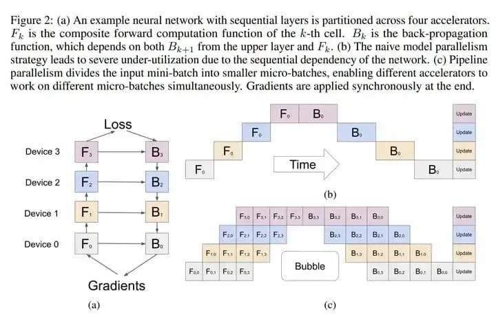
Micro batch effect

The report evaluated the effectiveness of micro batches in both the key value cache pre fill stage and the decorating stage (as explained in 2.2 Model Architecture). In the case of 4096 input tokens and 256 output tokens, the report found that micro batches improved inference throughput at the same local batch size, as shown in the following figure.

These improvements are attributed to micro batches achieving concurrent execution in these two stages. Due to the additional synchronization points brought by micro batches, latency increases, but overall, micro batches still provide a better throughput latency trade-off.

4.2 Quantization

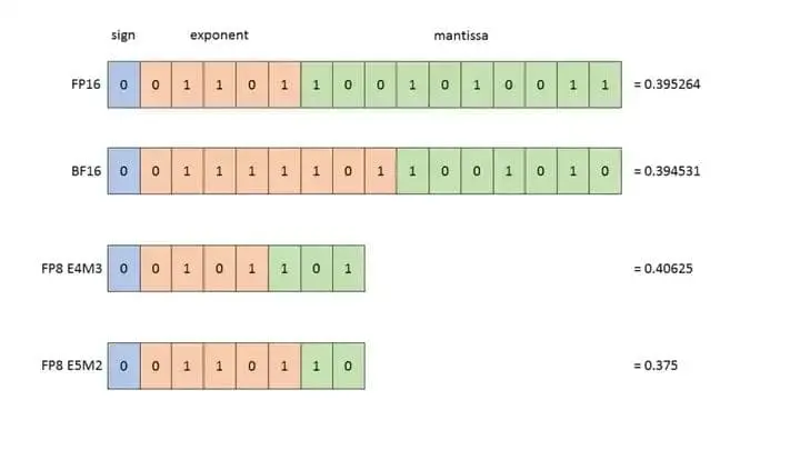
Quantization， Quantification is also a current hot topic, and the core approach is to reduce GPU usage and computational complexity by lowering the accuracy of model parameters. Similar to PagedAttention, there are also many related things that can be found in the OS. Some common precision representations are as follows:

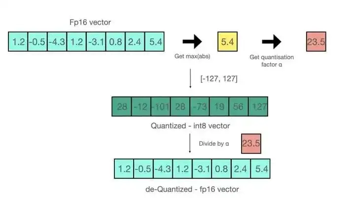
INT8 quantification

INT 8 quantization is relatively simple. The INT 8 quantization of absmax is shown in the figure, and the input is a FP16 vector. Assuming the vector [1.2, -0.5, -4.3, 1.2, -3.1, 0.8, 2.4, 5.4] is quantized using absmax. Firstly, the maximum absolute value of the vector needs to be calculated, which is 5.4 in this example. The range of Int8 is [-127, 127], so we divide 127 by 5.4 to obtain a scaling factor of 23.5. Finally, multiply the original vector by the scaling factor to obtain the final quantized vector [28, -12, -101, 28, -73, 19, 56, 127].

To restore the original vector, we can divide the int8 quantization value by the scaling factor, but due to the rounding process, we will lose some accuracy.

FP8 quantization

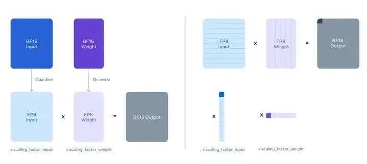
Llama 3 utilizes the native FP8 support of H100 GPU to perform low precision inference. To enable low precision inference, Llama 3 applies FP8 quantization to most matrix multiplications within the model. Please refer to the following two reference articles for implementation details. Especially, quantifying most of the parameters and activation values of the feedforward network layer in the model, which account for approximately 50% of the inference computation time. There are also some details among them:

Llama 3 did not quantify the parameters in the self attention layer of the model. Quantization was not performed in the first and last Transformer layers either. And, a row wise quantization method was adopted to calculate the scaling factor for each row of the parameters and activation matrix. As shown in the following figure.

Quantitative results

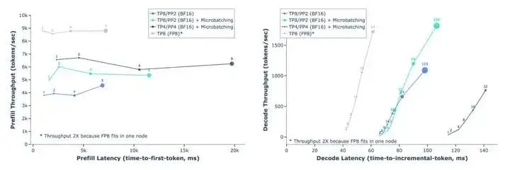
The quantitative results mainly have two aspects, one is the benefits, namely the improvement of efficiency; One disadvantage is the decrease in accuracy.

efficiency，Llama 34,096 input tokens and 256 output tokens，prefill（2.2 Model Architecture ），FP850%（4k->9k）；decode，trade off throughput-latency。

For accuracy, on a standard benchmark, even without the details mentioned earlier, the performance of FP8 inference is comparable to BF16 inference. However, when the Scaling Factor has no upper limit, the model sometimes generates incorrect responses, so the benchmark cannot accurately and fully reflect the impact of FP8 quantization. So Llama 3 used FP8 and BF16 to generate 100000 responses and chose to analyze them using the distribution of the reward model. From the figure below, it can be seen that the score of FP8 has almost no impact on the score distribution of RM.

Throughput-latency trade-off in FP8 inference with Llama 3 405B

Reward score distribution for Llama 3 405B using BF16 and FP8 inference.

Write 5 at the end

Recently, I have been busy with my work, so I spent about three weekends completing this nearly 20000 word article. I feel like there are many shortcomings after finishing writing, but I decided to post it at some random time. One reason is that the original plan was to start with high-quality open-source models and reports like Llama 3 to sort out some knowledge, but the writing almost retained the original structure of the paper, resulting in a lack of smoothness from one knowledge point to the next;

Secondly, due to insufficient proficiency and limitations in “comprehensiveness” considerations, there is a lack of detailed knowledge for many areas that require in-depth exploration. In the coming weekends, we may continue to iterate this article, mainly to further refine the technical points. So I also kindly request you to point out any errors or shortcomings and freely propose the parts that need to be supplemented.

Reference link

[1] IFEval Dataset | Papers With Code: https://paperswithcode.com/dataset/ifeval
[2] LiveBench: https://livebench.ai/
[3][KV Cache Optimization] MQA/GQA/YOCO/CLA/MLKV Notes: Intra layer and Inter layer KV Cache Sharing:https://zhuanlan.zhihu.com/p/697311739
[4]Hands on Deep Learning PyTorch Edition: Key Notes:https://zhuanlan.zhihu.com/p/664880302